The 6-step guide
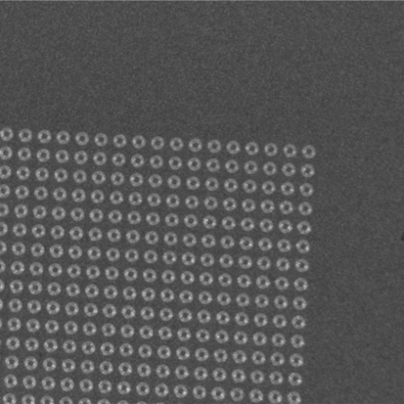
1) Grating mounting
Mount the grating in an X-ray Microscope equipped with FiberScanner3D™ module.
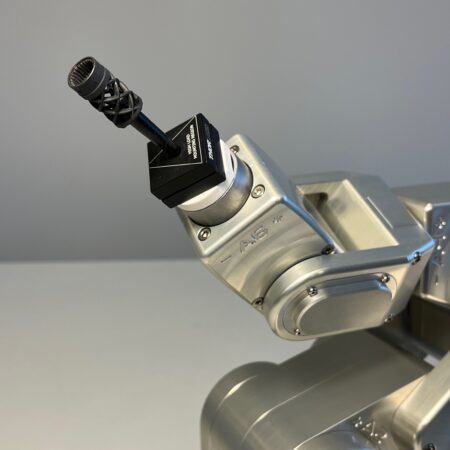
2) Sample mounting
Mount your component on the high-precision 6-axis robot arm using a quick-release mounting base.
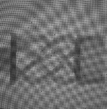
3) Data collection
Acquire the two data sets simultaneously:
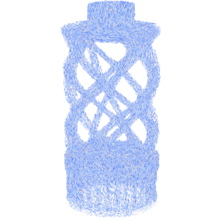
- Absorption contrast for sample outline and defects
(voids, inclusions, etc.) - Scattering contrast for fiber map reconstruction
4) Processing
Acquire data directly in Xnovo’s FiberScanner3D software.
Follow the step-by-step guide in the Graphical User Interface to
1. Select region of interest
2. Preview scattering signal
3. Launch 3D scan
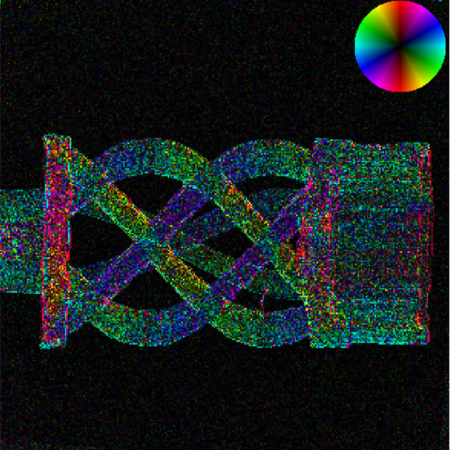
5) Reconstruction
As the reconstruction progresses, the full scattering tensor of the sample is generated.
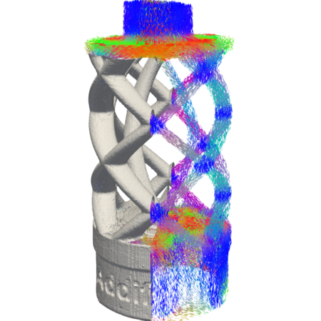
6) Results
Fiber orientation, degree of alignment, and relative fiber content are extracted alongside the full absorption contrast reconstruction.
