The 6-step guide
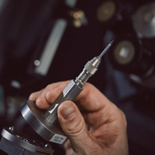
1) Sample mounting
Mount sample material in a Zeiss Xradia CrystalCT or a ZEISS Xradia 520/620 Versa X-ray Microscope equipped with a LabDCT Pro™ module.
Align the sample and choose aperture and beam stop to match the region of interest.
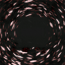
2) Data collection
Acquire two data sets:
- Absorption contrast for sample outline, voids and precipitates
- Diffraction contrast for grain map reconstruction
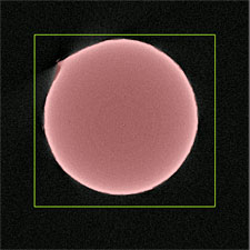
3) Processing
Load the acquired data into Xnovo’s GrainMapper3D software and enter basic information about the material. Follow the step-by-step guide in the Graphical User Interface to
- Select region of interest
- Separate signals from background
- Choose optimal reconstruction parameters
- Launch the 3D reconstruction
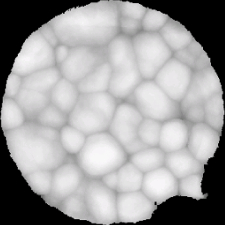
4) Reconstruction
As the reconstruction algorithm finds an indexing solution, a grain is added to the preview. The reconstruction process is converged once a space-filling 3D map is obtained.
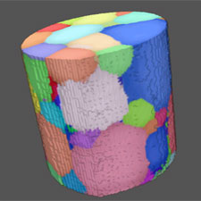
5) Results
Visualize the grain structure of the material in 3D. Colour coding can be chosen according to e.g. orientation, grain size, or completeness.
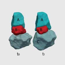
6) 4D evolution studies
Expose the sample to external stimuli such as heat or mechanical loading and repeat above steps to study the evolution of the microstructure.
